

How To Name X And Y Axis In Excel

MS Excel 2007: Create a nautical chart with two Y-axes and one shared X-axis
This Excel tutorial explains how to create a chart with two y-axes and one shared 10-axis in Excel 2007 (with screenshots and step-by-step instructions).
Question: How do I create a chart in Excel that has ii Y-axes and ane shared X-axis in Microsoft Excel 2007?
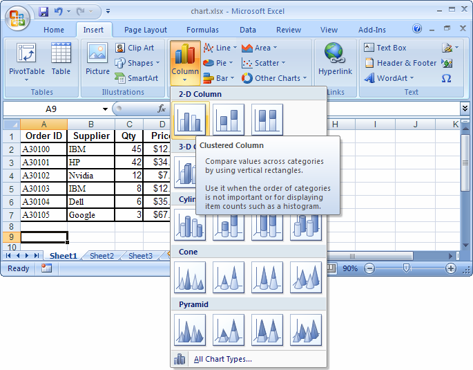
Answer:First, select the Insert tab from the toolbar at the top of the screen. In the Charts group, click on the Column button and select the kickoff chart (Amassed Column) under two-D Column.
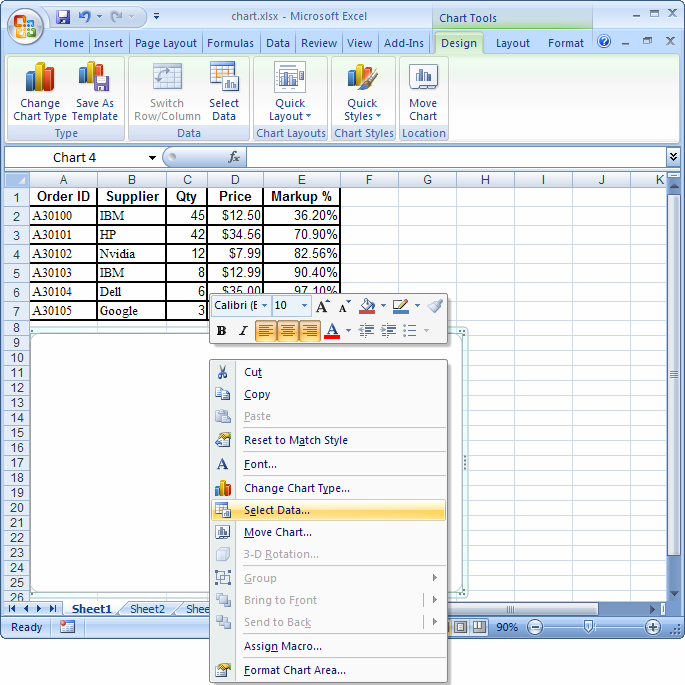
A blank chart object should appear in your spreadsheet. Right-click on this chart object and choose "Select Information..." from the popup card.
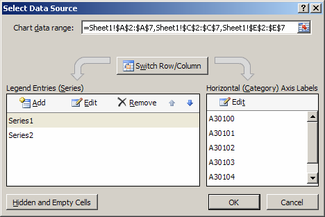
When the Select Data Source window appears, we need to enter the data that we want to graph. In this case, nosotros want cavalcade A to represent our Ten-centrality and column C to represent our principal Y-axis (left side) and column E to represent our secondary Y-centrality (correct side). Ane more complexity to this example is that our data is not all in adjacent cells, so nosotros need to select columns A, C, and E separated by commas.
To do this, highlight cells A2 to A7 then blazon a comma, then highlight cells C2 to C7, then blazon another comma, and the highlight cells E2 to E7. Yous should meet the following in your Chart data range box:
=Sheet1!$A$2:$A$seven,Sheet1!$C$2:$C$7,Sheet1!$E$2:$East$7
Click on the OK push button.
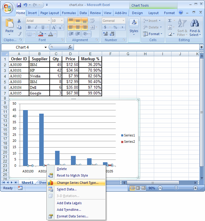
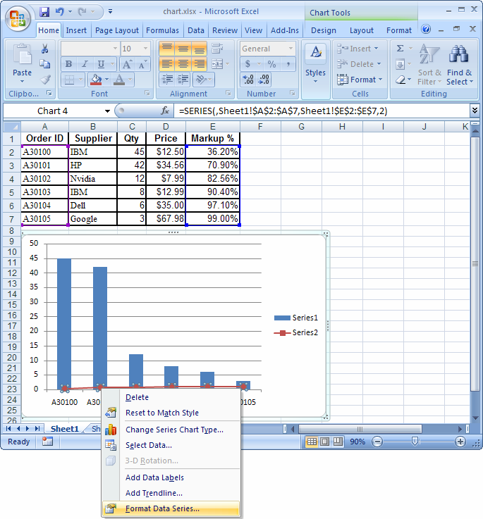
At present, correct-click on one of the data points for Series2 and select "Change Series Chart Type" from the popup menu.
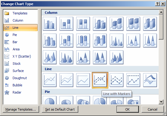
When the Change Nautical chart Type window appears, select the 4th nautical chart under the Line Chart section. Click on the OK button.
Now when you view the chart, yous should meet that Serial two has changed to a line graph. Nonetheless, we still demand to prepare a secondary Y-centrality as Serial 2 is currently using the principal Y-centrality to brandish its information.
To do this, correct-click on one of the data points for Series two and select "Format Data Series" from the popup menu.
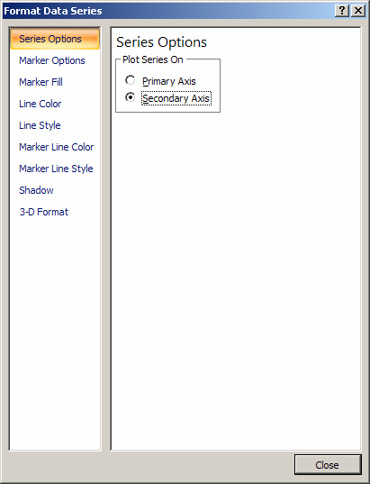
When the Format Data Series window appears, select the "Secondary Axis" radio push. Click on the Shut push.
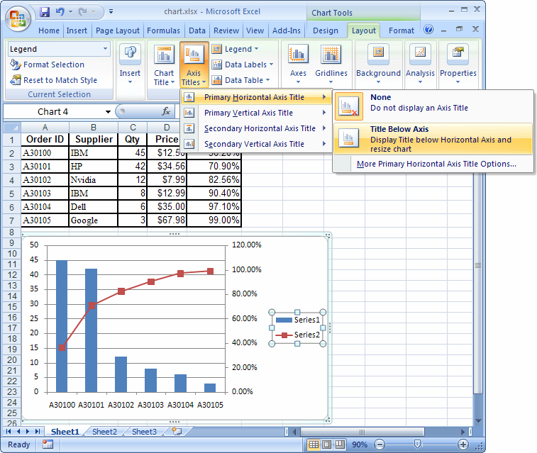
Now, if you want to add together axis titles, select the chart and a Layout tab should appear in the toolbar at the meridian of the screen.
Click on the Layout tab. Then select Axis Titles > Primary Horizontal Axis Championship > Championship Below Axis.
An Axis Title at the lesser of the graph should announced, merely overwrite "Axis Title" with the text that you'd like to run across.
Side by side, nether the Layout tab in the toolbar, select Axis Titles > Main Vertical Centrality Title > Horizontal Championship.
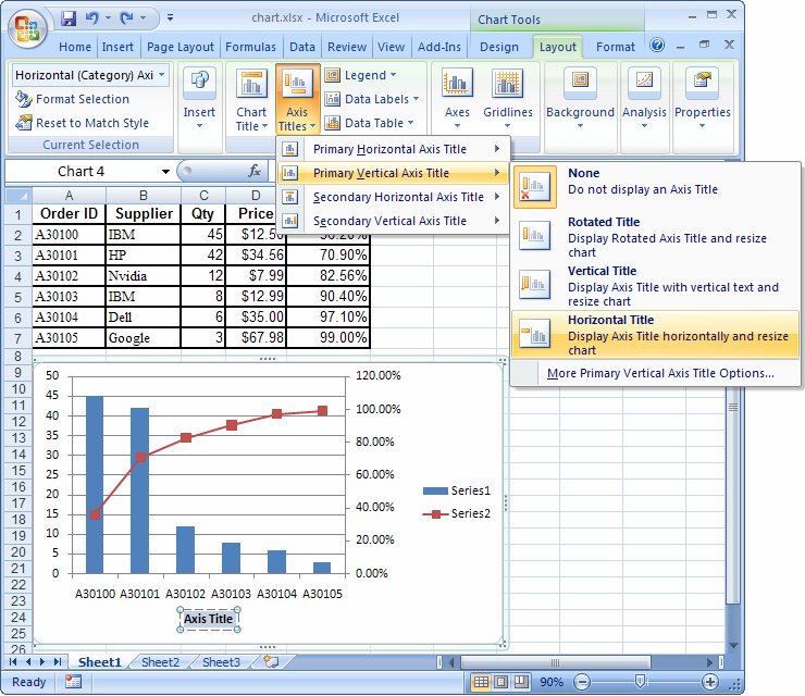
An Centrality Championship to the left of the graph should appear, just overwrite "Centrality Title" with the text that you'd like to encounter.
Side by side, under the Layout tab in the toolbar, select Centrality Titles > Secondary Vertical Axis Title > Horizontal Championship.
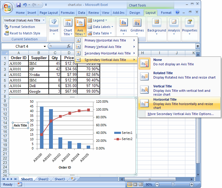
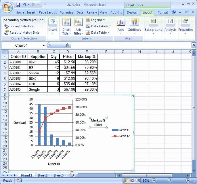
At present, you should see that your nautical chart is designed with a mutual Ten-axis and ii dissimilar Y-axes.

Source: https://www.techonthenet.com/excel/charts/2_y_axes.php
Posted by: bookercantences88.blogspot.com
0 Response to "How To Name X And Y Axis In Excel"
Post a Comment